Detecting waves in radial velocity#
Alongside the lake breeze model, AIDAS can detect wave signatures in Doppler radial velocity. This is not a machine learning product: it is the algorithm of Miller et al. (2022), and it works by subtracting two consecutive radar volumes from one another.
The idea is that the background wind changes very little over one volume cycle, while a propagating wave moves a long way in the same time. Subtracting the two sweeps therefore cancels the background and leaves the wave behind, as bands of alternating velocity change. AIDAS keeps the negative half of that difference, which marks the upstream convergence and the ascent implied with it, and turns it into a binary mask.
Before any of that, each sweep is quality controlled as the paper describes: gates with reflectivity below 0 dBZ are discarded, speckles are removed, and the velocities are dealiased with Py-ART’s region-based unfolding. The dealiasing is not optional in spirit. A fold is a jump of twice the Nyquist velocity, so an unfolded field is full of apparent velocity changes of 50 m s-1 or more sitting along the fold edges, and those would be detected in place of the waves. On the 2010 case below, roughly a fifth of the gates need unfolding, which takes the field from the ±26 m s-1 the radar reports out to −65 to 74 m s-1.
Running the detector#
The detector needs two scans. If you only give it one, it fetches the volume before it for you. The case the paper demonstrates the method with is KOKX at Upton, New York, late on 26 December 2010, with a low centre a couple of hundred kilometres to the southeast:
import aidas

rad_scan = aidas.model.detect_velocity_waves(
    'KOKX', rad_time='2010-12-26T23:45:15', max_range=137000.)
You can also hand it both scans yourself, as Py-ART radar objects, file paths, or a
RadarImage() you have already preprocessed:
rad_scan = aidas.model.detect_velocity_waves(later_scan, earlier_scan)
The result carries velocity_wave_mask, where 1 marks a detection, along with the
grid it sits on in wave_grid_lat and wave_grid_lon, and the two sweep times
that were differenced in wave_scan_times – here 23:40:00 and 23:45:48, the pair
the paper works from. Note that the wave mask lives on its own Cartesian grid centred
on the radar, at 0.5 km spacing by default, rather than on the 256 by 256 domain grid
the lake breeze mask uses.
To see it:
aidas.vis.visualize_velocity_waves(rad_scan)
(Source code, png, hires.png, pdf)
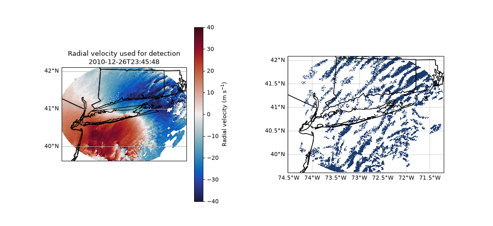
The mask is drawn in a panel of its own rather than as a contour over the velocity,
because band spacing and orientation are much easier to read that way. Beside it is
the velocity the detection actually worked from – the dealiased, quality controlled
sweep held in wave_sweep_radar, not the raw folded field in the original volume,
so the two panels agree with one another. Its colour scale runs past the Nyquist
velocity for the same reason. Pass overlay=True to outline the mask on the
velocity panel as well, which is the quick way to check that detections sit on the
bands they came from.
Checking the result against the paper#
Taking a two dimensional Fourier transform of that mask puts the dominant sets at wavelengths of 14 to 19 km with their long axes running 28 to 39 degrees, SSW to NNE, and the wave train moving off to the northwest. The paper reports wavelengths on the order of 12 to 18 km with SSW to NNE axes for the same case. Several roughly parallel bands moving together like this are what a wave train looks like, and what distinguishes it from a single boundary.
Tuning the detection#
The defaults are the WSR-88D values from the paper: flag velocity changes below -1 m s-1, grid at 0.5 km, and throw away detections covering less than 16 km2.
rad_scan = aidas.model.detect_velocity_waves(
    'KOKX', rad_time='2010-12-26T23:45:15',
    velocity_threshold=-1.0, grid_spacing=500., min_area=16.)
Of the three, min_area is the one worth thinking about. Waves exist at many
scales at once, so the area filter is not only removing noise – it is choosing which
wave scale you see. It is easiest to see by running the same case three ways, with
aidas.vis.plot_velocity_wave_mask() drawing each mask on its own:
import cartopy.crs as ccrs
import matplotlib.pyplot as plt

fig, axes = plt.subplots(1, 3, figsize=(15, 5),
                         subplot_kw=dict(projection=ccrs.PlateCarree()))

for ax, min_area in zip(axes, (0.25, 16., 400.)):
    rad_scan = aidas.model.detect_velocity_waves(
        'KOKX', rad_time='2010-12-26T23:45:15', max_range=137000.,
        min_area=min_area)
    aidas.vis.plot_velocity_wave_mask(
        rad_scan, ax=ax, title=f"min_area = {min_area:g} km$^2$")
(Source code, png, hires.png, pdf)
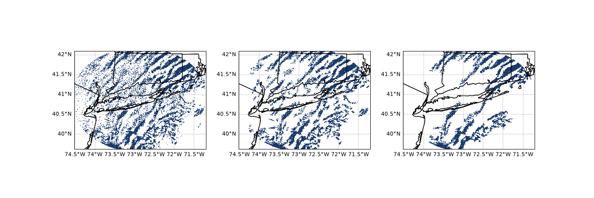
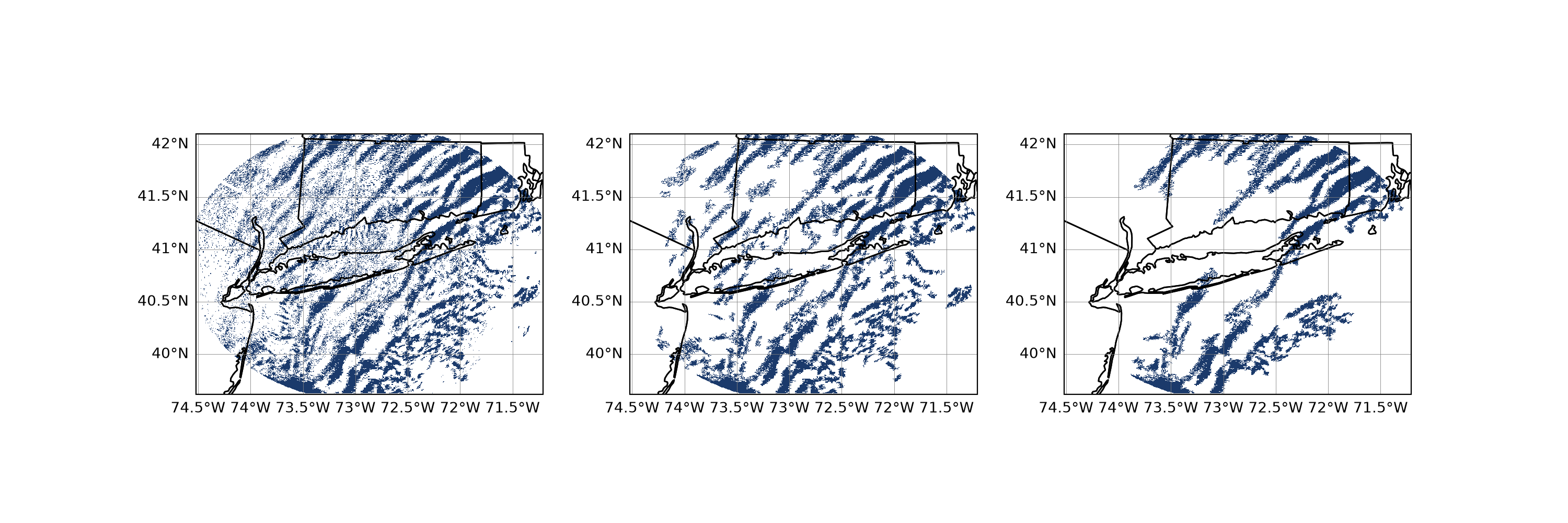
At 0.25 km2, a single grid cell, nothing is filtered at all and speckle covers the domain along with the waves. At the default 16 km2 the bands stand clear of it. At 400 km2 only the longest and most coherent bands survive and the shorter waves embedded among them are gone, which is the point: the filter is a choice about scale, not only about noise. The detected area falls from about 19 500 km2 to 15 600 and then to 10 100 across the three.
The paper reports that the result is not very sensitive to the exact velocity threshold for high-amplitude waves, and thresholds for other instruments should scale with their noise floor.
What the mask can and cannot tell you#
Two limits are worth keeping in mind.
The first is sampling. A wave has to move at least one resolution volume between scans to show up at all, and it has to move less than half a wavelength for its speed and direction to come out right:
With a roughly four minute volume cycle, a 10 km wave has to be travelling slower
than about 21 m s-1. Faster than that and the wave train appears to
stand still, flash in place, or move backwards. Clear-air volume coverage patterns
can take ten minutes to come round again, which makes the limit tighter still.
wave_scan_times holds the times of the two sweeps that were actually
differenced, so the interval can be checked rather than assumed. A pattern running
SAILS revisits the lowest elevation part way through each volume, but AIDAS takes the
base cut from both volumes, so the interval is one full volume cycle.
The second is interpretation. Any linear convergence feature is flagged, not just waves: gust fronts, sea and lake breezes, fronts, and terrain effects all produce a band. Those advect with the mean wind. A wave train instead looks like several roughly parallel bands moving together, and may move independently of the prevailing flow. Confirming that such a train really is a gravity wave takes evidence this mask does not carry.
The paper makes that point with a second KOKX case, the winter storm of 1 February 2021, which AIDAS will happily detect:
rad_scan = aidas.model.detect_velocity_waves('KOKX', rad_time='2021-02-01T09:03:09')
It produces strong banding in both the rain and the snow, but the bands stay locked to the precipitation structures and move with them, so the paper attributes them to mesoscale convergence rather than to waves. The mask cannot tell the two apart; that is the reader’s job.
Pointing an instrument at a wave train#
The pointing utilities take the wave mask as readily as the lake breeze mask:
angle, lat, lon, dist = aidas.util.azimuth_point(
    instrument_lon, instrument_lat, rad_scan, mask='velocity_wave')
aidas.util.azimuth_from_ellipse() is often the better choice here, since a wave
train of parallel bands fits an ellipse far more naturally than a single front does,
and it returns an azimuth across the bands rather than along them.